The workload behind the schedule, before it reaches the site.
A resource-loaded schedule carries its workload hour by hour and trade by trade, with key quantities such as concrete in m³, steel in tonnes and piping in WDI. Reading all of it takes an export, a pivot table and a chart, again at every update. In ploteer the workload sits under the schedule, and seven charts read it: the manpower per month with its S-curve, the peaks a steady crew cannot follow, the critical load, the bow wave, the trades stacked, the density and where the hours sit. Ready to present.
- Tell the site how many people it needs next month, trade by trade.
- Validate hours and FTE versus key quantity targets.
- Check the resource loading before the update goes out.
- Find the peaks a steady crew cannot follow, before they reach the site.
- See the months the critical path needs people.
- Review a resource-loaded schedule from the other side of the table: is the workload real, or pushed to the right?
- Put the workload on the screen for the progress meeting.
- 1
Import the XER. The resource assignments come as P6 holds them, and the workload sits under the schedule: all labour, or the trades you pick.
- 2
Open the charts from Report, and read the workload seven ways, each with its reading.
- 3
Click where the hours sit, and the schedule shows that work.
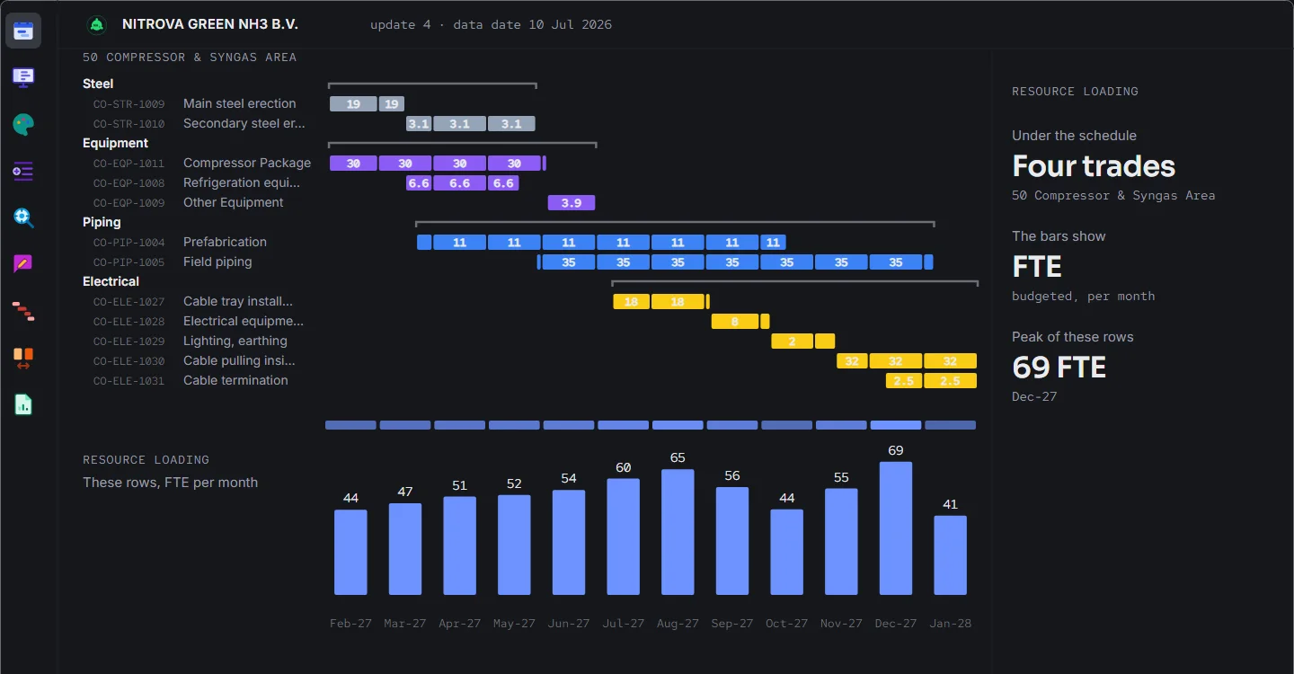
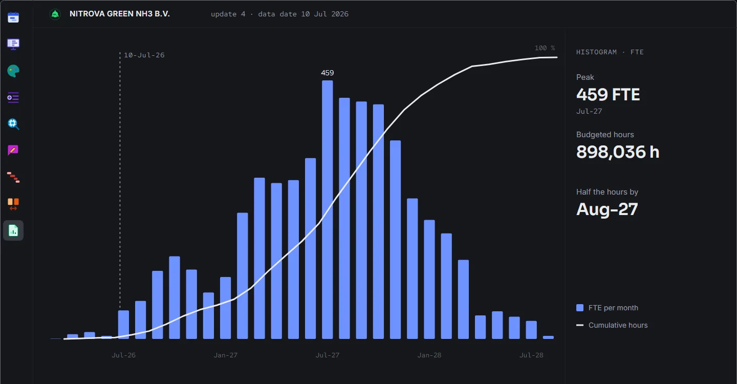
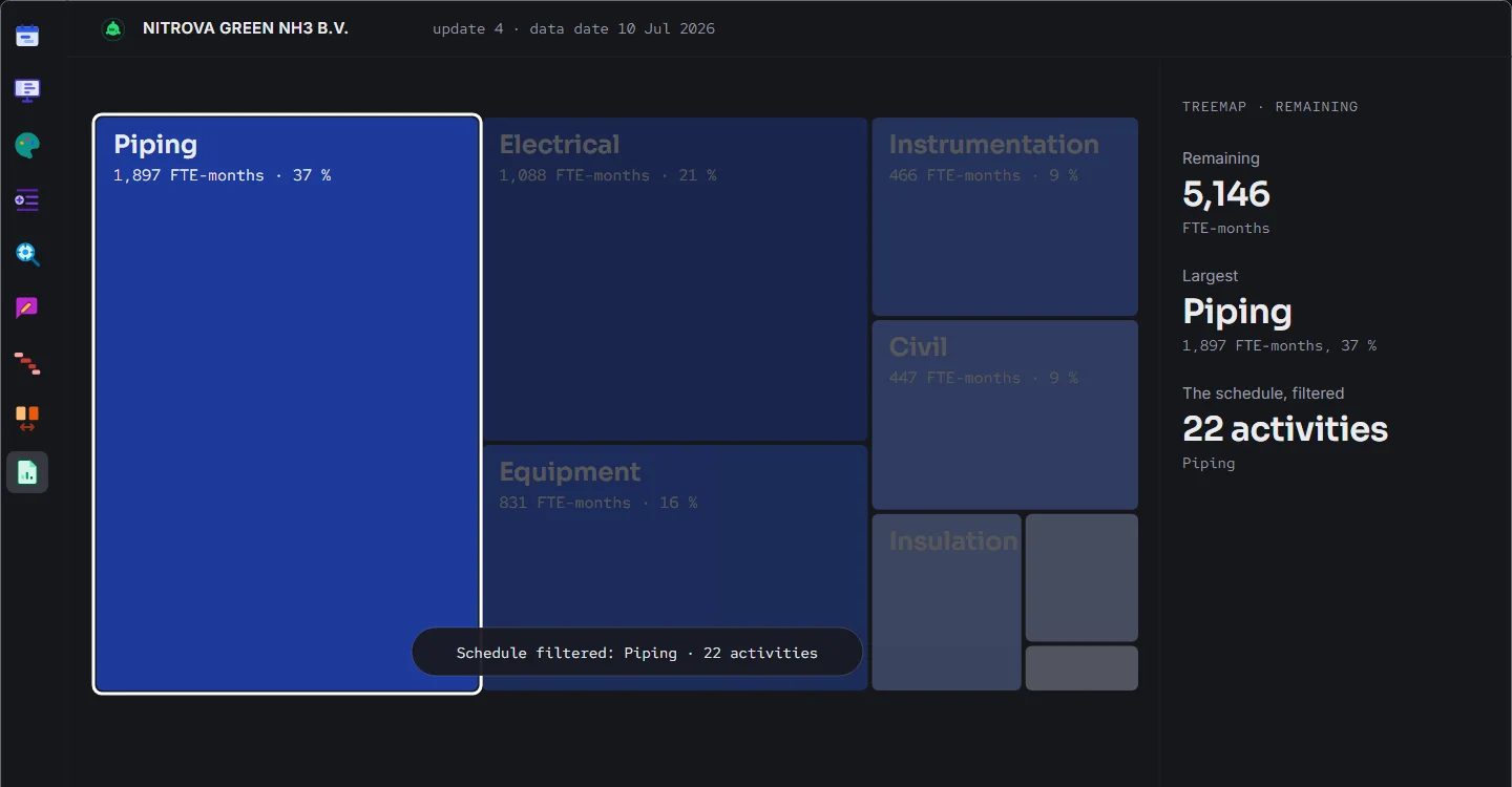
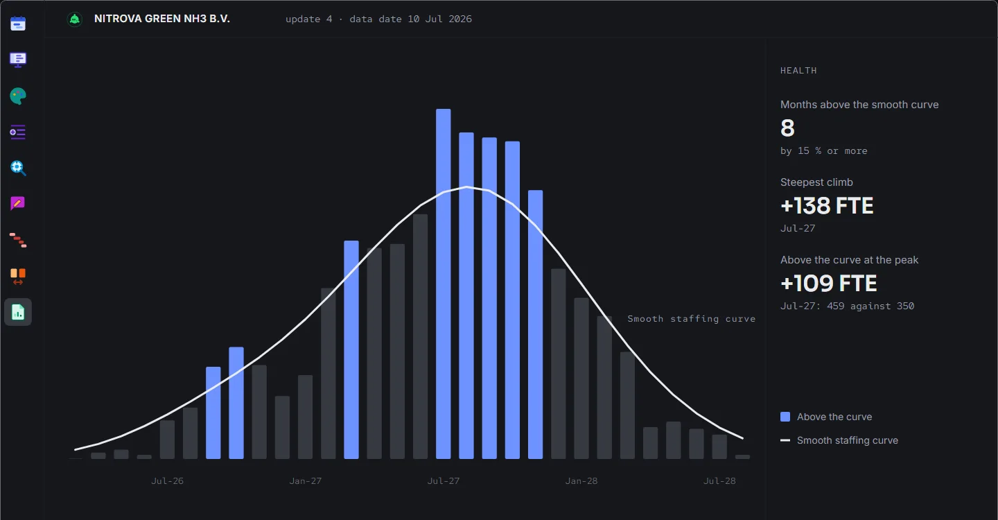
The workload of the schedule, read in one sitting.
The resource loading sits under the Gantt, on the same timescale: the bars above, the workload below. All labour, all non-labour or the resources you pick, per period, with a density view that shows where the load gathers.
Seven charts read the same workload. The histogram gives the manpower per period in FTE, with the S-curve of the hours, and reads the key quantities too: concrete in m³, steel in tonnes, piping in WDI. Health sets it against a smooth staffing curve, and the peaks a steady crew cannot follow stand out. Criticality colours each period the way the bars are coloured: done, critical, near-critical, on track. On the demo project, 32 % of the hours sit on critical work.
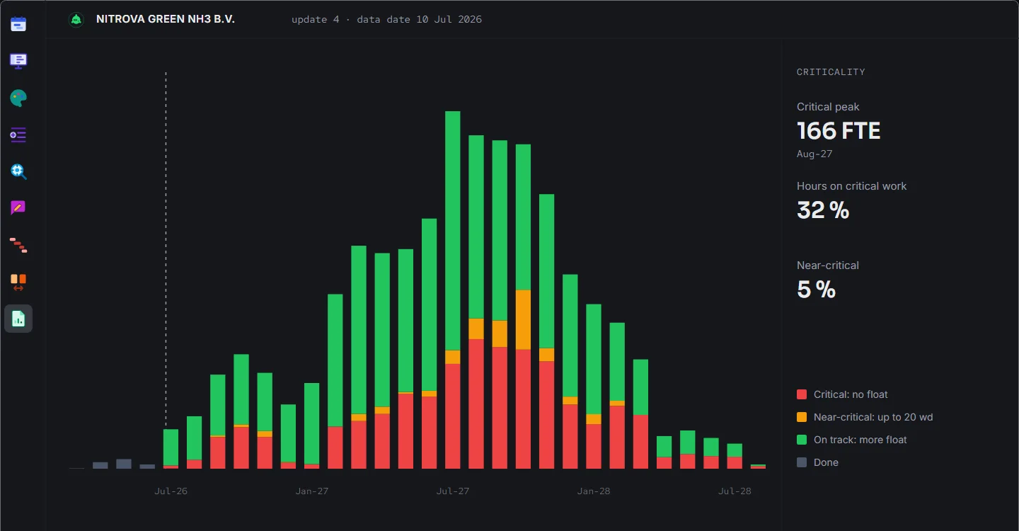
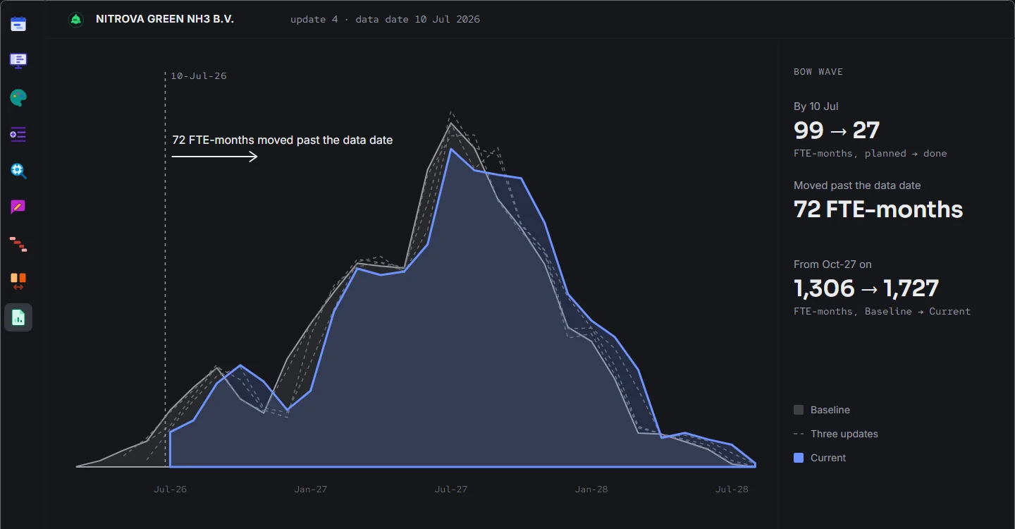
The bow wave sets the Current against the schedules before it. On the demo project the Baseline planned 99 FTE-months of work by 10 July 2026, and 27 are done. The other 72 moved past the data date, and the back end grew: from October 2027 on, the Current carries 1,727 FTE-months where the Baseline had 1,306. The total barely moved; the timing did. Dated update by update and exported as a PDF, the chart is a record: for the Client questioning a recovery the workforce cannot reach, and for the Contractor showing its plan is realistic, before anyone argues who carries the delay.
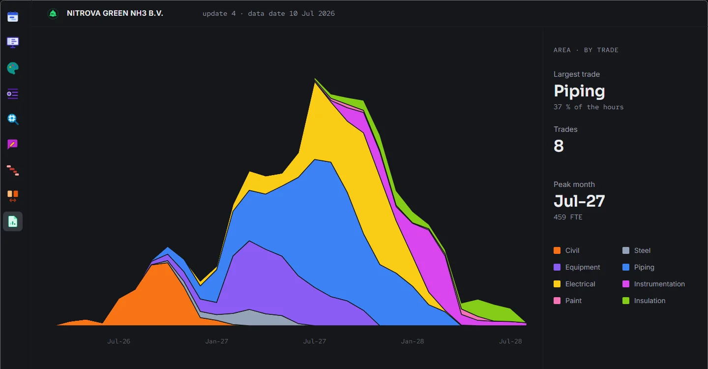
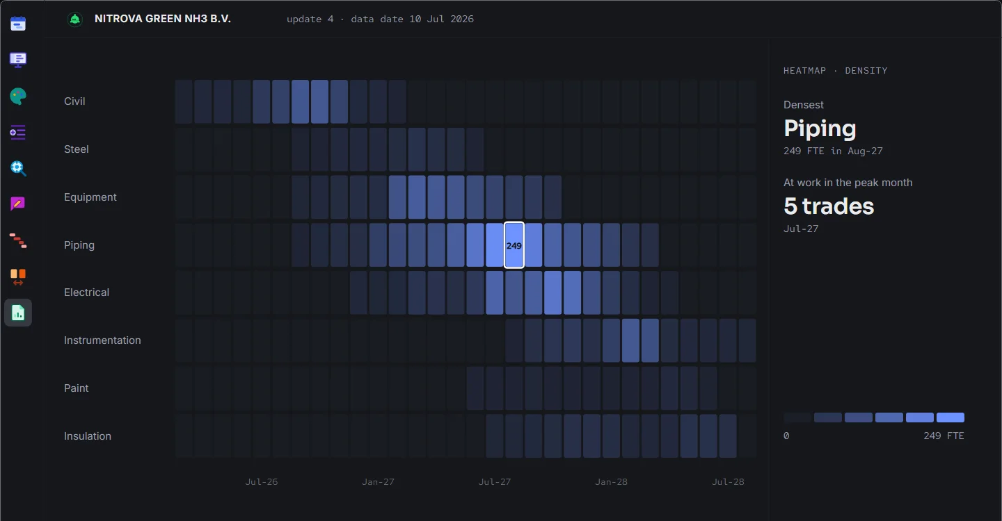
The area stacks the trades. The heatmap shows the density: a row per trade, a column per period, and the denser the work, the brighter the cell. The treemap shows where the remaining hours sit, and a click on a tile filters the schedule to that work.
Every chart goes out as a picture, a PDF or a presentation, in the light or the dark look, and to a spreadsheet with its own data table. Outputs tells the rest.